How to Predict Consumption Using Machine Learning Algorithms

Following last week’s post , which served as an introduction to Machine Learning algorithms, we will now carry out a consumption prediction. Starting from past consumption data, we will attempt to predict future values and see how well the prediction matches reality.

To do this, we will analyze the available data, what seasonality is and how it affects learning algorithms, and finally the choice of algorithm and its implementation in the R language.

Machine Learning – Consumption Prediction

The ultimate goal of this series of posts is to get ahead of future events and, in doing so, be able to anticipate the resources a company needs to handle both peaks and troughs in sales.

What data do we need to make predictions using Machine Learning algorithms?

We have sales data grouped by month, ranging from the earliest, in June 2014, to the most recent, in January 2017, so we aim to make a 9-month prediction. We also have actual data for the months between February and October 2017 so that, once the prediction has been made, we can compare it with the actual results.

Stationary series and series with seasonality

Studying the time series available is one of the most complex parts of the process of selecting a prediction algorithm.

The first step is to determine whether the series is stationary or not (stationary series or non-stationary series). The vast majority of prediction algorithms are designed to make predictions on stationary series, so it’s very important to understand what a stationary series looks like. As shown in this link, you can identify graphically whether your series is stationary or not. There are three criteria for classifying whether a series is stationary or not:

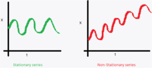
• The mean of the time series must not depend on time, meaning it must remain constant. As shown in the attached image, the green graph corresponds to the stationary series, where we can see that the mean is constant, while in the red graph we can see that the mean increases over time.

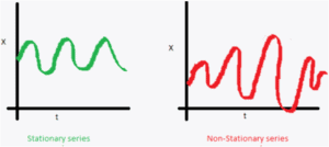
• The variance of the time series must be constant, meaning it must not change over time. As in the previous case, the green graph would correspond to a stationary series, as opposed to the non-stationary one in red. In the first, the variance is constant, while in the second the variance changes over time, since, as can be seen, the difference between the maximum and minimum values is greater in the central area of the red graph.

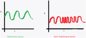
• The last criterion relates to the covariance between a point “i” in the time series and the point “(i+m)”. At these points, the covariance must remain constant over time. As can be seen, the red graph does not meet this requirement, since it “shrinks” and “stretches” over time, while the green graph has all its maximum and minimum values at the same distance apart.

Another important point when applying a prediction algorithm is determining whether the series has seasonality (seasonal series or non-seasonal series). In other words, it’s important to deseasonalize the series in order to remove periods of higher or lower sales, such as the summer or winter seasons.

After studying the consumption shown in the first graph, it’s easy to see that this series is not stationary and also lacks pronounced seasonality; sales are simply lower in August and December.

Due to the properties identified in the previous process, the algorithm we will use is found in the R statistical program, specifically the “auto.arima” function. This R function works with both stationary and non-stationary series, as well as series with or without pronounced seasonality.

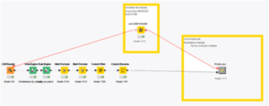
Finally, we will use Knime with R integration. Here you can find another post related to Knime and R. Below is an image showing what the graphical interface would look like in Knime:

Arima as a prediction algorithm

Therefore, to make a sales prediction when only past sales data is available, an easy-to-use algorithm is the Arima algorithm. As mentioned earlier, to use this algorithm we rely on the R function “auto.arima”. This function works with both stationary and non-stationary series, as well as series with or without pronounced seasonality. For all these reasons, this R function is the one chosen to carry out this prediction.

Coming up in the next post…

In next week’s post, we will present the results graphically and compare the prediction made with the actual consumption during the months evaluated.