
PCA Algorithm: From Complex to Simple
When faced with a complex situation, the goal is always to simplify the problem.
The PCA algorithm aims to simplify the initial problem to solve it from the simplest to the most complex form, while gaining the necessary experience to resolve the original issue.
PCA, Variable Reduction
Starting from a problem with multiple variables, the objective is to understand the relationship between them. To do this, the first step is to reduce the available variables as much as possible. Once this step is achieved, we represent the obtained result visually to observe how the data is grouped in an easy and intuitive way.
A CSV file is available that stores the history of purchase orders for certain parts. The objective of this data analysis is to group parts that, due to their characteristics, are close to each other—that is, located near each other in space. Doing this in a 12-dimensional space is neither simple nor graphically representable. To achieve this, the aim is to reduce the number of variables to the smallest possible number. To carry out this change, it was decided to use a mathematical technique known as “Principal Component Analysis.”
What is “Principal Component Analysis” or PCA, and what is it for?
It is a mathematical method used to reduce the number of variables so that we move to having a minimum number of new variables that represent all the old variables as accurately as possible. In other words, if the number of variables is reduced to two or three new ones, the original data can be represented on a plane or in a 3D graph, thus providing a visual summary of our data. The simple fact of having visible data greatly simplifies understanding what might be happening and helps in decision-making.
Next, we proceed with the analysis of the purchase orders. We will not go into purely mathematical details due to their complexity.
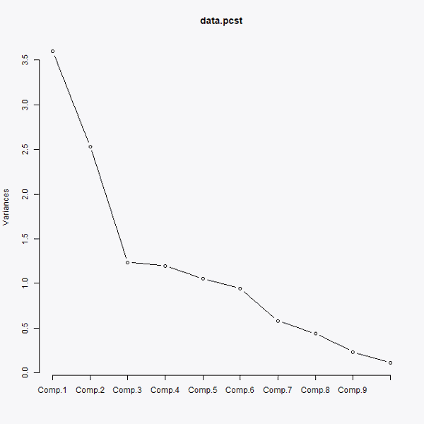
The very first step is to observe, through the following graph, how many principal components we should select.
Choosing the number of principal components
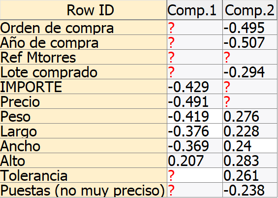
As seen in the previous graph, the first three components account for the most variance, so we can say they are the main components for performing the analysis. However, to represent the results two-dimensionally throughout this post, we will choose only the first two. In the following graph, we can see the influence each variable exerts on the new principal components:
Influence of each variable on the two principal components
As we can observe, the variables that exert the most weight on the first of the principal components are the measurements of the parts, while the variables that exert the most weight on the second of the principal components are the rest of the variables, with the year of purchase and the purchase order number having a greater influence. It could be said that the first principal component represents the characteristics of the parts purchased, while the second principal component represents the properties of the purchase.
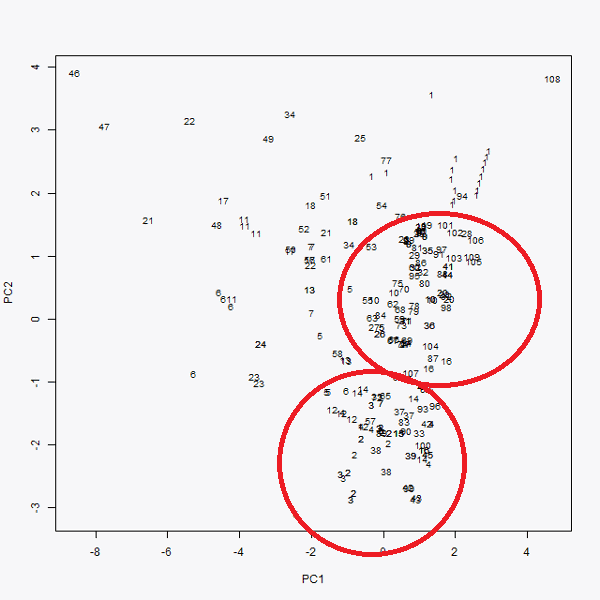
Once the representation of each variable is known, they are represented in two dimensions. The first of the principal components is plotted on the ‘x’ axis and the second on the ‘y’ axis. This produces Graph 3, where the representation of the initial data in two dimensions can be observed.
In this way, an interpretation of each purchase order can be made. It can be seen that purchase order number 46 (top left in Graph 3), as well as purchase 108 (top right), could be considered outliers. However, what is most striking about this graph is that more than 80% of the data is condensed into two groups, highlighted by two red circles. This indicates that the purchase orders not close to these groups are the ones causing a greater variance in the price of the purchase orders. The further to the right a purchase order is, the more expensive it should be, and the further to the left it is located, the cheaper it must be. We deduce this from Graph 2 and how each variable influences the principal components.
Graphic representation in the two principal components
Data classification using the K-Means algorithm
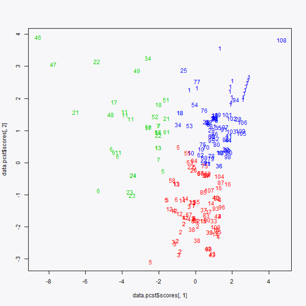
Once this graphic representation is completed, we move on to using the K-means algorithm. This algorithm is used to locate groups within a “point cloud,” which in this case are the purchases. It has been decided to group the data into three groups; therefore, the K-means algorithm is being performed with K=3. The result obtained is as follows:
K-means graph
Consequently, three groups are obtained. As mentioned earlier, there were two clearly differentiated groups (now one in red and the other in blue), and we located a third group formed by the rest of the points representing all the data that “falls outside” the two previously mentioned purchase order groups.
To continue the analysis and draw deeper and more important conclusions, an in-depth analysis would need to be performed on the data of the third group, represented in green.
Conclusion
When faced with a multitude of variables to analyze, it is best to reduce these variables to a minimum to represent them graphically and intuitively. Once this step is done, other techniques can be applied, as in this case, which serve to understand even more clearly and explicitly how to use the data or how to interpret it.
This type of data analysis is very useful for relating variables to each other and understanding their connections. Applied to logistics, for example, this study can also be used to decide the best geographical location for a warehouse. If we consider the points in the last image as final customers and plan to build three warehouses to distribute a company’s products, we can determine that the optimal location for the warehouses would be in the center of each of these groups, ensuring that the distance from the warehouse to the customers is minimized.
Share on Facebook
Share on Google
Share on Twitter
Share on LinkedIn
Share on Pinterest
Share on Print
Share on Email