Automated Demand Prediction

Automated Demand Prediction

How much material do we need to purchase in the coming weeks? When will we need to produce a specific product? Do we have sufficient capacity to meet demand? These are some of the questions businesses strive to answer daily. Demand prediction for your products is essential for efficient planning within companies and can provide the optimal solution to these questions. It is common to have hundreds of products for which demand needs to be known at least monthly. Even when fewer forecasts are required, there may be no one sufficiently trained in the use of predictive models. In these circumstances, an automatic forecasting algorithm can be a very valuable tool.

Predictive Algorithms

Generally, there are two types of methods for making predictions: qualitative methods and quantitative methods. While qualitative methods, such as the Delphi method, are based on expert knowledge and opinion, quantitative methods use past data within mathematical models to make predictions. In cases involving a new product for which no data exists, or in strategic projects where many factors are important, qualitative methods may perform better. However, with the availability of more data and increased computational capabilities, quantitative methods are becoming more common. Furthermore, these methods can be automated and do not depend on expert knowledge. Therefore, we will describe some quantitative methods in detail.

Predictions are a research area with a long tradition, and a large number of models and algorithms have been developed. Nevertheless, due to significant differences in demand between products, no single model is perfect for predicting all products. This is why at LISDATA, we use different predictive algorithms to ensure predictive quality. The methods can be grouped into the following families:

• Naive Methods.
• Exponential Smoothing Methods.
• ARIMA Methods.
• Other Methods.

All of these rely solely on historical demand data to calculate predictions. Their adjustment for each product can be automated, making them ideal for automating predictions.

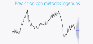
Naive methods are very simple and use historical values for prediction. One such method is the basic Naive method, where the prediction corresponds to the last observed value. Another method is the seasonal Naive method, which uses the value from the same period of the previous year as the prediction. Although these methods are often not very precise, there are situations where their use can be appropriate. For example, they are frequently used in the financial sector.

Exponential Smoothing methods are based on the component model of time series. In this model, the time series is divided into trend, seasonality, and an error component, which are extrapolated to create the prediction. Future values are calculated using recursion formulas where the last value is combined with a moving average of historical values. These methods are very common and are particularly suitable for predicting demand driven by clear trends and seasonality.

Prophet is an algorithm based on the same ideas. It was developed by Facebook engineers. Similar to Exponential Smoothing methods, the time series is divided into components, additionally allowing for the inclusion of holiday and seasonal influences at multiple temporal levels. The different components are modeled using various functions (logistic growth, Fourier series, auto-regressions). This algorithm can predict demands with overlapping seasonal patterns, meaning patterns that integrate with each other, and trends at hourly (website visit prediction), daily, or weekly levels.

Similar to Exponential Smoothing methods, ARIMA models have a long tradition in time series and demand forecasting. These models combine auto-regressive (AR) and moving average (MA) models with integrated (I) data. Auto-regressive models represent a linear combination of short-term past values. Moving average models combine past random factors. For proper functioning, the data must be stationary. To eliminate potential trends or seasonality, the data is integrated. These factors are re-added at the end of the calculation. ARIMA models are suitable for time series where the influence of short-term past values is significant.

With these different types of methods, it is possible to predict all types of demand on a daily, monthly, or annual basis. By automating the algorithms, these predictions can be calculated regularly without any manual interaction.

Choosing the Optimal Method

All these methods have their strengths and weaknesses. Using only one of these algorithms would not lead to a satisfactory result. So, when should we use which method? This question can sometimes be answered by observing the demand time series and its characteristics. However, this is impossible if thousands of predictions are needed. For these cases, we can generate a classification model created with Machine Learning algorithms. Machine Learning algorithms (e.g., Support Vector Machine or Classification Trees) are fed with historical metadata that includes, on one hand, the characteristics of the time series (strength of trend, seasonality, autocorrelation, entropy, etc.) and, on the other hand, the optimal method for each time series. Machine Learning algorithms recognize relationships between the characteristics of the time series and the optimal method, thereby creating a classification model. This classification model can be applied to any time series and its characteristics to determine the method to apply for prediction.

Evaluating Predictions

By using multiple prediction methods and always choosing the most appropriate one, we optimize predictions and minimize their error. However, it is not possible to eliminate error completely. For this reason, it is essential to calculate the prediction error so that the user can evaluate the prediction and its reliability. With the help of cross-validation of the chosen prediction method, we can estimate the future prediction error. To calculate the prediction error, test predictions are calculated within the historical data. These test predictions are compared with the available data, calculating the estimated error of the actual prediction.

By defining limits for the prediction error, it is possible to assess whether the prediction is reliable or not. Additionally, predictive algorithms calculate confidence ranges that also convey the reliability of the prediction.

At LISDATA, we develop automated systems with different prediction methods that can regularly predict the demand for thousands of products, minimizing prediction error and transparently communicating their reliability. With this information, we can know when we should produce, which product, or how much material we should purchase. Ultimately, we optimize planning, increasing its efficiency and reducing costs.

For more information, contact us at info@lisdatasolutions.com